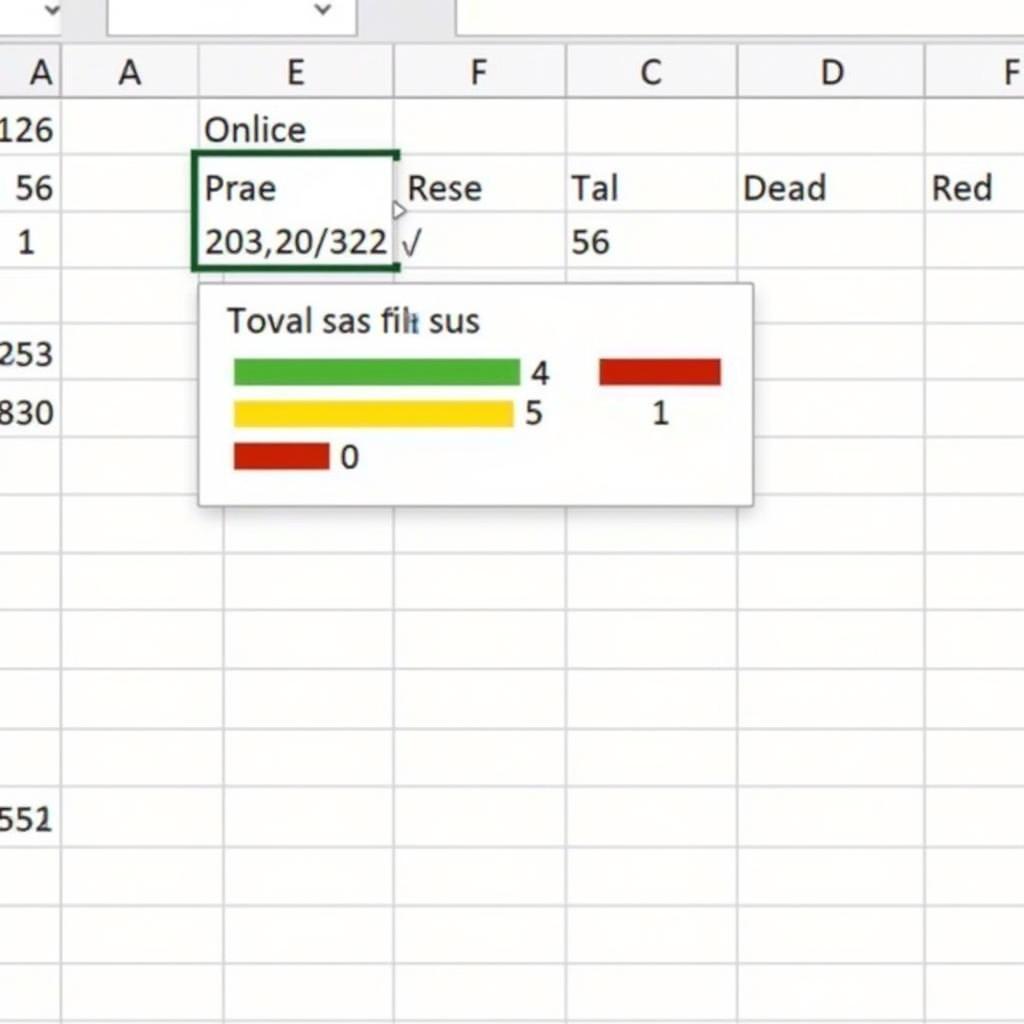
How to Conditionally Format Cells in Excel

Conditionally formatting cells in Excel is a powerful technique that allows you to easily track and analyze data. Instead of reading each cell individually, you can use colors to highlight important values, trends, or anomalies.

Applying conditional formatting in Excel

Basic Steps to Conditionally Format Cells in Excel

Excel provides a Conditional Formatting feature that lets you apply color rules automatically. Here are the basic steps:

1. Select the data range: Highlight the cells you want to conditionally format.
2. Open Conditional Formatting: Go to the Home tab, and in the Styles group, select Conditional Formatting.
3. Choose a rule: Excel offers a variety of pre-defined formatting rules. Common rules include:
   • Highlight Cells Rules: Highlight cells based on their values (greater than, less than, equal to, between…).
   • Top/Bottom Rules: Highlight the highest, lowest, or top/bottom values.
   • Data Bars, Color Scales, Icon Sets: Add data bars, color scales, or icons to cells based on their values.
4. Set up the rule: After selecting a rule, you need to define specific criteria. For example, if you choose the “Greater Than” rule, you need to enter a value to compare against.
5. Choose a format: Select the colors, font styles, or other formats to apply to cells that meet the criteria.

Example of conditional formatting in Excel

Examples of Conditional Formatting in Excel

1. Highlight Cells Greater Than or Less Than a Specific Value

• Choose the Greater Than or Less Than rule in Highlight Cells Rules.
• Enter the value you want to compare against.
• Select the format you want to apply.

2. Highlight Cells Containing a Specific Keyword

• Choose the Text that Contains rule in Highlight Cells Rules.
• Enter the keyword you want to search for.
• Select the format you want to apply.

3. Highlight Cells Based on the Value of Another Cell

• Choose the Use a formula to determine which cells to format rule.
• Enter a formula that compares the value of the current cell with another cell.
• Select the format you want to apply.

For example, to highlight cells in column A that are greater than the corresponding values in column B, you can use the formula =$A1>$B1.

Tips for Effective Conditional Formatting

• Use meaningful colors: Choose colors that are relevant to the data context. For example, use red for negative values and green for positive values.
• Combine multiple rules: You can apply multiple formatting rules to the same data range.
• Use the rules manager: To view and edit applied rules, go to Conditional Formatting > Manage Rules.

“Mastering Conditional Formatting can save you time and effort in data analysis,” says Nguyen Van A, a data analyst at [Company Name].

Conclusion

Conditional formatting is a powerful tool in Excel that allows you to easily identify patterns, trends, and important data points. By applying simple techniques, you can transform your spreadsheets into more visual and effective tools.

FAQ

1. Can I copy conditional formatting to other cells? Yes, you can use the Format Painter to copy conditional formatting.
2. How do I remove conditional formatting from a data range? Select the data range, go to Conditional Formatting > Clear Rules > Clear Rules from Selected Cells.
3. Can I use Excel functions in conditional formatting formulas? Yes, you can use most Excel functions in conditional formatting formulas.

Learn More About:

• Conditional Formatting
• How to Conditionally Format Cells in Excel
• How to Color a Cell in Excel

Contact Us Today!

For the best advice and support on XE TẢI HÀ NỘI services, please contact:

• Phone: 0968239999
• Email: [email protected]
• Address: No. TT36 – CN9 Road, Tu Liem Industrial Park, Phuong Canh Ward, Nam Tu Liem District, Hanoi.

We have a 24/7 customer service team ready to assist you.